Credit card fraud detection with data storytelling: from rare-event EDA to a threshold the ops team can defend

Start with the business reality, not the model

Before any algorithm runs, the data already tells an operational story. A fraud ops team does not care about ROC curves — they care about how many transactions came through, how many were fraud, and how much was at stake. The training window covers 227,845 transactions over about 48 hours, including 394 confirmed fraud cases. Fraud is 0.173% of the stream. That imbalance is not a side note; it is the central constraint that shapes everything downstream, because a model can look 'accurate' while still missing the exact rare events the business cares about.

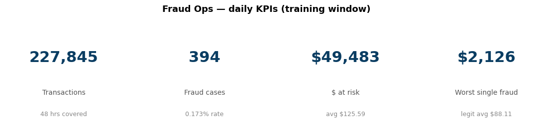
The dollar context matters just as much. The same slice carries roughly $49,483 in fraud exposure with a worst-single-fraud of $2,126, so the question is never just 'how many frauds are caught?' but also 'which fraud dollars are recovered, and which expensive misses still slip through?'

EDA as the backbone — where fraud actually lives

EDA here is not a checklist of charts. It is the part that makes the fraud problem legible. The first strong signal is temporal: normal transaction volume rises through the commercial day, but fraud rate spikes overnight — the early-morning window that usually reflects automated card testing rather than real spending behaviour.

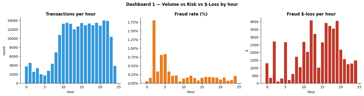
The split between rate and dollars is one of the most important insights in the project. A rate-based alert wakes ops at 2 a.m. for testing patterns; a dollar-based alert points instead at the 10am–8pm window where higher-value fraud blends into legitimate activity. Both are correct — they answer different questions.

hourly = query("""
    SELECT CAST((Time/3600) % 24 AS INTEGER) AS hour,
           COUNT(*)                                       AS n,
           SUM(Class)                                     AS frauds,
           100.0*SUM(Class)/COUNT(*)                      AS fraud_pct,
           SUM(CASE WHEN Class=1 THEN Amount ELSE 0 END)  AS fraud_dollars
    FROM t GROUP BY hour ORDER BY hour
""", t=train)

Amount risk — fraud is not the big-ticket event you think it is

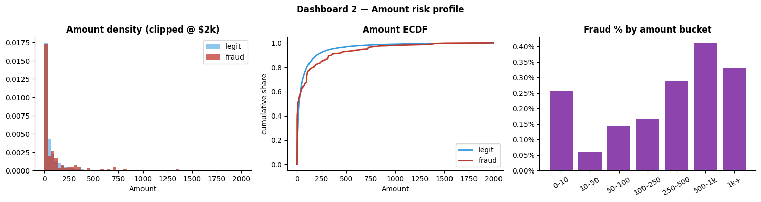
The amount analysis adds a second layer. Fraud is not concentrated only in large purchases; much of it appears in low-value transactions consistent with stolen-card validation. But the fraud rate also rises again in the $500–$1,000 range, which means blanket filters based on 'large' or 'small' amounts would miss part of the real risk structure.

Where the signal lives — feature-level storytelling

Of the anonymised PCA features V1–V28, only a handful carry the fraud signal. Correlation analysis isolates V17, V14, V12 and V10 as the dominant negative correlates, and V11 and V4 as the strongest positives. The violin plots confirm visible class separation — the precondition for any model to work at all.

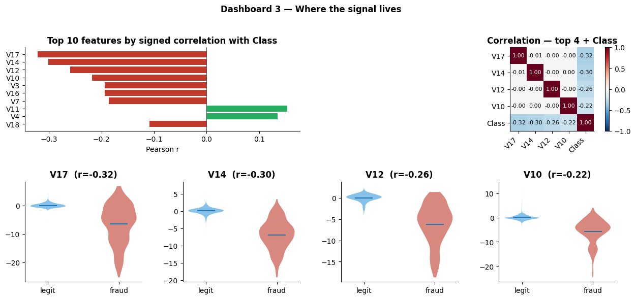
Later, SHAP attribution on the trained model points at the same group of features. That alignment between exploratory EDA and post-hoc model attribution is itself an audit signal: the model is learning the structure already visible in the data, not memorising noise.

The review-budget curve — operating policy before model choice

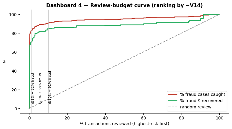
If we ranked transactions by a single feature's 'fraud-ness' and gave analysts a fixed daily review budget, how much fraud could we catch? This is the view ops actually plans against. Sorting by −V14 alone — no model yet — catches 82% of fraud at 1% review volume, and 91% at 10%. A one-feature rule already crushes random review.

Explain the ML simply — boosted trees, calibrated, thresholded by dollars

The champion model is XGBoost — a gradient-boosted tree model that improves performance by building many small decision trees in sequence, each new tree focusing on the mistakes the previous ones made. That matters in fraud because fraud behaviour is rarely linear: a suspicious transaction is usually defined by an interaction between latent behaviour patterns, timing and amount, and boosted trees are good at capturing those non-linear combinations.

Raw boosted-tree scores rank transactions well but are not numerically reliable as probabilities. So the project calibrates with Platt scaling on validation, then sweeps the threshold by net dollars saved (recovered fraud dollars − analyst review cost) instead of using 0.5 by default. The pipeline in plain English: split first so leakage cannot happen, fit preprocessing only on training data, train the ranker, calibrate on validation, then pick the cutoff using business cost.

Make the metrics tell a story

On the held-out test set the numbers are strong, but they become much more compelling when narrated as decisions rather than results. The model delivers $2,496.73 in net savings versus a no-model baseline, recovers 64.0% of fraud dollars, catches 89.8% of fraud cases at a calibrated cutoff of 0.1875, reaches 73.33% precision overall, and lands PR-AUC 0.8855 / ROC-AUC 0.9774 with Precision@100 = 0.45.

Segment-level robustness — does the average hide a failing slice?

Overall PR-AUC of 0.886 is a single number. The interesting question is whether it holds across slices the analyst will actually see — different hours of day, different amount buckets — or whether one cohort drags the average up while another silently fails.

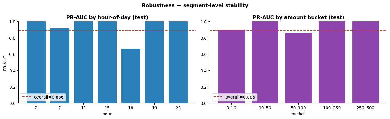
• Most hour-of-day slices hold at PR-AUC 0.9+ — the model generalises across the daily cycle.
• The 6pm hour drops to PR-AUC 0.66 — a concentrated population of confusing transactions, worth investigating before production.
• Across amount buckets, only $50–$100 dips below the overall line, and only slightly.

What this project does differently

1. Split before transform. Stratified train/val/test partitions are created before any scaler, encoder, or feature step runs — leakage is impossible by construction.
2. Class imbalance handled, not ignored. No naive SMOTE-everything. scale_pos_weight in XGBoost preserves the legitimate class while up-weighting the rare one during gradient computation.
3. Calibrate before thresholding. Raw boosted-tree probabilities are poorly calibrated; Platt scaling on validation makes the threshold sweep meaningful in dollar terms.
4. Threshold by net savings. The chosen 0.1875 cutoff is the argmax of (recovered_fraud_dollars − analyst_review_cost) on validation, not a default.
5. Explain every alert. SHAP values per prediction tell analysts which features drove the score — V14 dominant, V4 supporting — turning the model into a defensible second opinion instead of a black box.

What to build next

• Cost-sensitive training. Pass Amount as the sample weight so the loss natively penalises missing a $2,000 fraud more than a $20 one. Expected lift: close the 26-point case-vs-dollar gap by 5–10 points.
• Time-aware validation. Replace random stratified split with a forward-rolling split that respects transaction time order — the only honest way to estimate next-week performance.
• Drift monitor. Track PR-AUC weekly per hour-of-day and per amount bucket. The 6pm dip in the robustness chart is the canary — it is the first metric that will move when the fraud pattern shifts.
• Analyst feedback loop. Every reviewed alert becomes a new labelled example; retrain monthly. Fraud models decay fast — quarterly is too slow.